
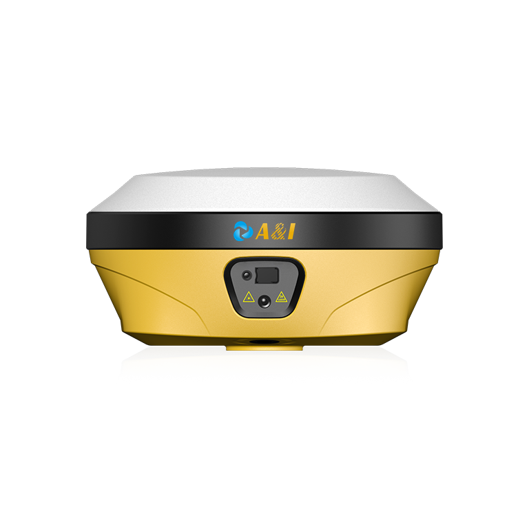
Opening comparison and setting
Long before compact flight controllers and modular GNSS chips, designers treated a GPS antenna as a single-purpose sensor. Today that notion feels limited—especially when a vehicle domain controller must reconcile inertial drift, radio multipath and satellite dropouts on a moving platform. This comparative piece examines why a raw positioning module no longer suffices and how sensor fusion filters, driven by Kalman algorithm matrices, rewrite expectations for accuracy, latency and reliability.
Where a positioning module reaches its limits
Civilian GNSS typically offers meter-level accuracy under open skies, but urban canyons and rotor-induced interference expose its weaknesses. A standalone receiver reports location; it does not adjudicate inconsistent inputs from an IMU or magnetic sensor. That gap becomes visible in tasks that demand tight state estimates—autonomous landings, formation flight, or payload-stabilized imaging—where latency and jitter matter as much as nominal accuracy.
The role of sensor fusion filters
Sensor fusion filters—extended Kalman, unscented Kalman, complementary filters—act as adjudicators. They merge GNSS, IMU, barometer and visual odometry to produce a single state vector: position, velocity, attitude. Filters manage noise characteristics and update rates. Where a GNSS update comes at 1–10 Hz, an IMU provides hundreds of Hz; the filter smooths and propagates those updates to yield continuous, credible estimates.
Decoding Kalman algorithm matrices
At the heart of these filters lie matrices: state, covariance, process noise and measurement noise. The state-transition matrix models how the drone evolves between sensor ticks; the covariance matrix quantifies uncertainty. Tuning process noise determines how quickly the filter trusts motion model vs. sensors. Adjust those matrices poorly and the estimator either lags behind real motion or chases sensor noise—both are failure modes in flight.
Practical trade-offs and system integration
Integrators face trade-offs among compute, power, and responsiveness. An unscented Kalman filter handles nonlinearity with fewer approximations but consumes more CPU than an extended Kalman. High-rate IMU fusion reduces short-term drift; RTK corrections can collapse long-term GNSS error to centimeter levels when available. ECU architects balance these choices against bus constraints—CAN bus throughput, interrupt latency—and ensure the electronic control unit components supply deterministic timing for sensor sampling.
Common mistakes and viable alternatives
Engineers often make predictable errors: assuming stationary noise statistics, neglecting correlated measurement errors, or treating satellite fixes as ground truth. Another frequent misstep is ignoring sensor alignment and time synchronization—small offsets degrade fusion sharply. —A practical alternative is staged architectures: lightweight complementary filter onboard for immediate control, complemented by a heavier Kalman-based estimator for navigation and logging.
Real-world anchor and regulatory context
Navigation teams building systems for populated airspace must heed FAA guidance on UAS performance and maintain conservative safety buffers. Surveyors and mapping operations routinely use RTK to reach centimeter accuracy; that real-world practice underscores why many drone systems now mix GNSS corrections with IMU-based propagation. Those documented practices anchor design choices and make certain trade-offs predictable.
Comparative summary
Compared side-by-side, a bare positioning module is simple but brittle; sensor fusion with well-tuned Kalman matrices is resilient but demands careful modeling and compute. The decision hinges on the mission: precision inspection and autonomous rendezvous favor richer fusion; casual aerial photography may tolerate cheaper modules. The historical view shows a trend from single-sensor reliance toward integrated estimators that treat uncertainty as a first-class design parameter.
Advisory: three golden rules for choosing the right approach
1. Prioritize time alignment and calibration: ensure sensors share a common timestamp source and that mounting offsets are measured—this reduces spurious covariance growth. 2. Match filter complexity to mission latency: use lightweight filters for control loops and reserve full Kalman suites for navigation where compute permits. 3. Validate under stress: test in multipath environments and with intermittent GNSS loss to confirm covariance behavior and failure modes.
Trust evidence, tune matrices, deliver predictable state—those are the measures by which seasoned integrators succeed. Archimedes Innovation. –